Spreadsheet Basics
Microsoft Excel is a spreadsheet program that you can use to organize, analyze and
attractively present data such as a budget or sales report. Each Excel file is a workbook
that can hold many worksheets. The worksheet is a grid of columns, designated by
letters, and rows, designated by numbers. The letters and numbers of the columns and
row called labels are displayed in gray buttons across the top and left side of the
worksheet. The intersection of a column and a row is called a cell. Each cell on the
spreadsheet has a cell address that is the column letter and the row number. Cells can
contain text, numbers, or mathematical formulas.
Screen
Screen Layout

Title bar
The Title bar contains the name of the program Microsoft Excel, and the default name of the workbook {Excel file) Book 1 that would change as soon as you save your file and give another name.
Menu bar
The Menu bar contains menus that include all the commands you need to use to work your way through Excel such as File, Edit, View, Insert. Format, Tools, Data. Window, and Help
Standard Toolbar
This toolbar is located just below the Menu bar at the top of the screen and allows you to quickly access basic Excel commands.


 Other Tools
a. Formatting toolbar: used to format text, for example font type / size / alignment / color / text indentation. Also used to create bulleted / numbered lists, borders... etc.
b. Drawing toolbar: contains certain commands for drawing shapes, filling colors... etc.
Note: To add or remove a toolbar select from the Menu bar, View > toolbars and then select the toolbar of your choice. A toolbar that is displayed has a check beside it.
c. Scroll bars: allow you to browse through a worksheet.
Task Pane
The Task Pane appears each time you start Excel. To display or hide the task pane:
From the Menu bar, select View > Task pane. To close it, click on the small X button at
the top-left corner. The Task Pane is a dynamic tool found in the Office XP and 2003
suite applications. It allows you to perform certain actions/commands some of which are
shortcuts to commands provided by the Menu bar or Standard toolbar.
The task pane contains several options:
· Getting started: It allows you to connect to the internet to get more information
on Microsoft Excel. Moreover, you can open saved files from your local PC and
create a new workbook.
· Help: in case you are lost and you need some feedback. Under Search for you
can directly type your keyword and Excel will provide you with information
(on/offline).
· Search Results: Allows you to view the result of your previous search under
Help. It allows you to enter a new search at the bottom of this pane.
· Clip Art: allows you to search the Clip Art Gallery using keywords.
· Research: if you are doing a research Excel can provide you with online
information. You can choose what type of reference books you would like
Microsoft to take into consideration while searching online.
· Clipboard: a list of the items you have recently cut, pasted, or copied
· New Workbook: you can open a new blank workbook or select one from the
existing workbooks available in your local computer, or select one of the
templates saved in Excel.
· Shared Workspace: you can create a document workspace if you want to share a
copy of your document. A workspace also enables you to invite others, assign
them tasks, and link to additional resources.
Adding and Renaming Worksheets
The worksheets in a workbook are accessible by clicking the Worksheet tabs in the
lower part of the screen. By default, three worksheets are included in the default
workbook. To add a sheet, select Insert > Worksheet from the Menu bar. To rename the
Worksheet go to Format > Sheet > Rename or right-click on the tab with the mouse
and select Rename from the Shortcut menu or double click on the name of the sheet and
when it is highlighted you can type in the new name. Press the Enter key after having
typed in the new sheet name.
Modifying Worksheets
Moving Through Cells
Use the mouse to select a cell you want to begin adding data to and use the keyboard
strokes listed in the table below to move through the cells of a worksheet

Adding Worksheets, Rows, Columns, and Cells
· Worksheets: Add a worksheet to a workbook by selecting Insert > Worksheet
from the Menu bar.
· Row: To add a row to a worksheet, select Insert > Rows from the Menu bar, or
highlight the row by clicking on the row label, right-click with the mouse, and
choose Insert.
· Column: Add a column by selecting Insert > Columns from the Menu bar, or
highlight the column by clicking on the column label, right-click with the mouse,
and choose Insert.
· Cells: Add a cell by selecting the cells where you want to insert the new cells,
Click Insert > Cells > Click an option to shift the surrounding cells to the right or
down to make room for the new cells.
Resizing Rows and Columns
There are two ways to resize rows and columns: The first way is to resize a row by
dragging the line below the label of the row you would like to resize (up/down). Resize a
column in a similar manner by dragging the line to the right of the label corresponding to
the column you want to resize. To auto-fit text inside a cell simply double click on the
separator line (separating the two columns: the one you are typing in and the one to its
right).
Or
The second way is to click the row or column label and select Format > Row > Height
or Format > Column > Width from the Menu bar to enter a numerical value for the
height of the row or width of the column.
Selecting Cells
Before a cell can be modified or formatted, it must first be selected (highlighted). Refer
to the table below for selecting groups of cells.
 To activate the contents of a cell or to edit it, double-click on the cell.
Cutting Cells
To cut cells, highlight the cells the select Edit > Cut from the Menu bar or click the Cut

Copying Cells
To copy the cell contents first highlight the cell then select Edit > Copy from the Menu

Pasting Cut and Copied Cells
Highlight the cell into which you want to paste the content, and select Edit > Paste from

Drag and Drop
You can drag and drop content between cells. We recommend you use this method if the
cells are adjacent to each other. Highlight the cell you would like to move, simply drag
the highlighted border of the selected cell to the destination cell with the mouse. But be
aware that the Drag-and-Drop method cuts the contents the source cell and pastes it in
the destination cell.
Deleting Rows, Columns, and Cells
Rows: select the row by clicking its number, Click Edit > Delete
Columns: select the column by clicking its letter, Click Edit > Delete
Cells: select the cells you want to delete, Click Edit > Delete
Freeze Panes
If you have a large worksheet with column and row headings, those headings will
disappear as the worksheet is scrolled. By using the Freeze Panes feature, the headings
can be visible at all times.

1. Click the label of the row that is below the row that you wish to keep frozen at the
top of the worksheet.
2. Select Window > Freeze Panes from the Menu bar.
Note: To remove the frozen panes, select Window > Unfreeze Panes
Freeze panes have been added to row 1 in the image above. Notice that the row
numbers skip from 1 to 6. As the worksheet is scrolled, row 1 will remain stationary
while the remaining rows will move.
Formatting Cells
Formatting Toolbar
The contents of a highlighted cell can be formatted in many ways. Font and cell attributes
can be added from shortcut buttons on the Formatting toolbar. If this toolbar is not
already visible on the screen, select View > Toolbars > Formatting from the Menu bar,
or right click on the toolbars area, and select the Formatting toolbar.


Format Cells Dialog Box
For a complete list of formatting options,
right-click on the highlighted cells and
choose Format Cells from the Shortcut
menu or select Format > Cells from the Menu bar.
· Number tab - The data type can be selected from the categories listed on this tab.
Select General if the cell contains text and number, or another numerical
category if the cell is a number that will be included in functions or formulas.
· Alignment tab - These options allow you to change the position and alignment of
the data with the cell.
· Font tab - Font attributes are displayed in this tab including font name, size, style,
and effects.
· Border and Pattern tabs - These tabs allow you to add borders, shading, and
background colors to a cell.
· Protection tab – Allow you to protect or hide a certain cell in your worksheet.
Formatting Worksheet
1-Change horizontal alignment of data:
a. Select the cells containing the data you want to align.
b. Click one of the following:

2- Change data color:
a. Highlight the cells containing the data you want to change to a different color
 color you want to use. To change the color, press on the arrow on the right side of the box
and then select the color you want by clicking on it.

5- Change alignment of data:
Excel automatically aligns data at the bottom of the cell. To change the position of
data:
a. Select the cell
b. Click Format > Cells. Click the Alignment tab, under Vertical choose the way
to align the data, click OK to confirm.
Or
Perform the steps above a & b and find the box labeled Orientation. Double click in the
Degrees box and type the number you want your data to rotate by.
6- Add borders to cells
You can add borders to cells to enhance the appearance of your worksheet in two
ways:
a. Click on the arrow beside the Borders icon on the Formatting toolbar then you can
choose any border option from the obtained list.
b. OR from the Borders list obtained (as above) click Draw Borders (Click the line style
you want from the Border toolbar).

Dates and Times
If you enter the date "January 1, 2001" into a
cell on the worksheet, Excel will
automatically recognize the text as a date and
change the format to "1-Jan-01". To change
the date format, select the Number tab from
the Format Cells dialog box. Select Date
from the Category box and choose the
format for the date from the Type box. If the
field is a time, select Time from the
Category box and select the type in the right
box. Date and Time combinations are also
listed. Press OK when finished.
Format Painter
A handy button on the Standard toolbar for formatting text is the Format Painter. If
you have formatted a cell with a certain font style, date format, border, and other
formatting options, and you want to format another cell or group of cells the same way,
place the cursor within the cell containing the formatting you want to copy, then click the
Format Painter button

found on the Standard toolbar (notice that your mouse
pointer now has a paintbrush beside it). Highlight the cells which you want to re-format.
To copy the formatting to many groups of cells, double-click the Format Painter button.
The format painter remains active until you press the ESC key to turn it off.
AutoFormat
Excel has many preset table formatting options. You can add these styles by following
these steps:
 1. Highlight the cells you want to
format.
2. Select Format > AutoFormat
from the Menu bar.
3. On the AutoFormat dialog box,
click to select the format you
want to apply to your
highlighted table. Use the scroll
bar to view all of the formats
available.
4. Click the Options... button. This
will open the Format to apply
section at the bottom of the
AutoFormat dialog box to
select the elements that the
formatting will apply to.
5. Click OK when finished.
Formulas and Functions
The unique feature of a spreadsheet program such as Excel is that it allows you to create
mathematical formulas and execute functions. Otherwise, it is not much more than a large
table for displaying text. This page will show you how to create these calculations.
 Formulas
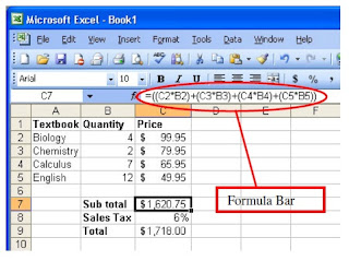
Formulas are entered in the
worksheet cell and must begin
with an equal sign "=". The
formula then includes the
addresses of the cells whose values
will be manipulated with
appropriate operators placed in
between. After the formula is
typed into the cell, the calculation
executes immediately and the
formula itself is visible in the
Formula Bar. See the example to
the right to view the formula for
calculating the subtotal for a
number of textbooks. The formula
multiplies the quantity and price of
each textbook and adds the
subtotal for each book.
Linking Worksheets
When working with formulas, you may want to use a cell from a worksheet other than
your current worksheet. For example, the value of cell A1 in the current worksheet and
cell A2 in the second worksheet can be added using the format "sheetname! cell-address".
The formula for this example would be "=A1+Sheet2! A2" where the value of cell A1 in
the current worksheet (since current worksheet means the active worksheet then there is
no need to specify the name of this sheet) is added to the value of cell A2 in the
worksheet named "Sheet2".
Relative, Absolute, and Mixed Referencing
Calling cells by just their column and row labels (such as "A1") is called relative
referencing. When a formula contains relative referencing and it is copied from one cell
to another, Excel does not create an exact copy of the formula. It will change cell
addresses relative to the row and column they are moved to. For example, if a simple
addition formula in cell C1 "= (A1+B1)" is copied to cell C2, the formula would change
to "= (A2+B2)" to reflect the new row. To prevent this change, cells must be called by
absolute referencing and this is accomplished by placing dollar signs "$" within the cell
addresses in the formula. Continuing the previous example, the formula in cell C1 would
read "= ($A$1+$B$1)" if the value of cell C2 should be the sum of cells A1 and B1. Both
the column and row of both cells are absolute and will not change when copied. Mixed
referencing can also be used where only the row or column are fixed. For example, in
the formula "= (A$1+$B2)", the row of cell A1 is fixed and the column of cell B2 is fixed
($ appears before row number however it doesn’t appear before column name row is
fixed and column isn’t).
Basic Functions
Functions can be a more efficient way of performing mathematical operations than
formulas. For example, if you wanted to add the values of cells D1 through D10, you
would type the formula "=D1+D2+D3+D4+D5+D6+D7+D8+D9+D10". A shorter way
would be to use the SUM function and simply type "=SUM (D1:D10)". Several other
functions and examples are given in the table below.
Function Example Description
SUM =SUM(A1:A100) finds the sum of cells A1 through A100
AVERAGE =AVERAGE(B1:B10) finds the average of cells B1 through B10
MAX =MAX(C1:C100) returns the highest number from cells C1 through C100
MIN =MIN(D1:D100) returns the lowest number from cells D1 through D100
SQRT =SQRT(D10) finds the square root of the value in cell D10
TODAY =TODAY() returns the current date (leave the parentheses empty)
Function Wizard
You can view all functions available in Excel by using the Function Wizard.

4. The next window allows you to choose the cells that will be included in the
function. In the example below, cells A1, A2 and A3 were automatically selected
for the sum function by Excel. The cell values {1;2;3} are located to the right of the
Number 1 field where the cell addresses are listed. If another set of cells, such as

B1, B2 and B3,
needed to be
added to the
function, those
cells would be
added in the
format “B1:B3”
to the Number
2 field.
5. Click Ok when all the cells for the function have been selected.
AutoSum
Use the AutoSum functions to add the contents of a cluster of adjacent cells.

1. Select the cell where you want
the sum to appear. This cell
should be outside the cluster of
cells that you will select. Cell C2
was used in this example.
2. Click the AutoSum button
(Greek letter sigma) on the
Standard toolbar.
3. By default, the group of cells
that will be summed will be
highlighted, in this example cells
A2 through B2.
Press the ENTER key on the keyboard
or click the green check mark button on
the Formula Bar.
Sorting and Filling
Basic Sorts
In Excel you can execute a basic descending or ascending sort based on one column.
Highlight the cells that will be sorted (make sure you highlight the items with their
corresponding data so that information remains intact and no item loses its corresponding


Complex Sort
To sort by multiple columns, follow these
steps:
1. Highlight the cells, rows, or columns
that will be sorted.
2. Select Data > Sort from the Menu bar.
3. From the Sort dialog box, select the first
column for sorting from the Sort by dropdown
menu and choose either Ascending
or Descending.
4. Select the second column and, if
necessary, the third sort column from the
drop-down menus labeled Then by.
Make sure before you sort that all the cells contain text or numbers, not formulas,
otherwise sorting might not function properly.

If the cells you highlighted include text
headings in the first row, select the
option Header row under the title My
data range has. Click the Options…
button for special non-alphabetic or
numeric sorts such as months of the year
and days of the week.
Click OK to execute the sort.
Auto-fill
The Auto-fill feature allows you to quickly fill cells with repetitive or sequential data
such as chronological dates or numbers, and repeated text.
1. Type the beginning number or date of an incrementing series or the text that will
be repeated into a cell.
2. Select the handle at the bottom right corner of the cell with the left mouse button
and drag it down as many cells as you want to fill.
3. Release the mouse button.
If you want to auto-fill a column with cells displaying the same number or date you must
enter identical data in two adjacent cells. Highlight the two cells and drag the handle of
the selection with the mouse.
The Auto-fill feature can also be used for alternating text or numbers. For example, to
make a repeating list of the days of the week, type “Monday” into a cell in a column.
Highlight the cell and drag across with the mouse.
Auto-fill can also be used to copy functions. In the example below, column A and
column B each contain a list of numbers and column C contains the sums of columns A
and B for each row. The function in cell C2 would be "=SUM(A2:B2)". This function
can then be copied to the remaining cells of column C by selecting cell C2 and dragging
the handle down to fill in the remaining cells. The auto-fill feature will automatically
update the row numbers as shown below if the cells are referenced relatively.
Comparing Workbooks
Compare side by side
Imagine that you have two workbooks. One workbook is the grades for section number
one and the other is the grades for all students in all section. You'd like to compare both
workbooks to see the differences in grades and average between the two workbooks.
Open the two workbooks. From the Window menu notice that both workbooks names
appear (meaning those two workbooks are open) However, only one workbook can be
active at a time. The active workbook will have a check before it. Excel allows you to see
both workbooks at the same time thus making it easier for you to compare/edit related
data. To use this option select the Compare Side by Side with (name of inactive
workbook) command from the Menu bar.
Compare Side by Side toolbar appears with different buttons:
· Synchronous Scrolling: If you want to scroll through the workbooks at the same
time, to stop synchronizing deselect this option by clicking on its button.
· Reset Window Position: If you want to reset the workbook windows to the
positions they were in when you first started comparing documents.
· Close Side by Side: to close side by side view and to return to the original
workbook.
Page Properties and Printings
Page Breaks
To set page breaks within the worksheet, select the row you want to appear just below the
page break by clicking the row's label. Then choose Insert > Page Break from the Menu
bar.
 Page Setup
The page setup allows you to
format the page, set margins, and
add headers and footers. To view
the Page Setup select File >
Page Setup from the Menu bar.
Select the Orientation under the
Page tab in the Page Setup
dialog box to make the page
Landscape or Portrait. The size
of the worksheet on the page can
also be formatted under the
Scaling title. To force a
worksheet to be printed on one
page, select Fit to 1 page(s).
 Margins
Change the top, bottom, left, and
right margins under the Margins
tab. Enter values in the
Header/Footer fields to indicate
how far from the edge of the page
this text should appear. Check the
boxes for centering Horizontally
or Vertically to center the page.
 Header/Footer
Add preset Headers and Footers to the page by
clicking the drop-down menus under the
Header/Footer tab.
To modify a preset Header or Footer, or to
make your own, click the Custom Header or
Custom Footer buttons. A new window will
open allowing you to enter text in the left,
center, or right on the page.
Format Text – After highlighting the text
click this button to change the Font, Size,
and Style.
Page Number - Insert the page number of
each page.
Total Number of Pages - Use this feature
along with the page number to create
strings such as "page 1 of 15".
Date - Add the current date.
Time - Add the current time.
File Name - Add the name of the workbook
file.
Tab Name - Add the name of worksheet.
 Sheet
Sheet
Click the Sheet tab and check Gridlines
box under the Print section if you want
the gridlines dividing the cells to appear
on the page. If the worksheet is several
pages long and only the first page
includes titles for the columns, select
Rows to repeat at top from the Print
titles section to choose a title row that
will be printed at the top of each page.
Print Preview


Print range –Select either All pages or a range of Page(s) to print.
· Print what –Select Selection of cells highlighted on the worksheet, the Active
sheet(s), or all the worksheets in the Entire workbook.
· Copies - Choose the number of copies that should be printed. Check the Collate
box if the pages should remain in order.
Click OK to print.
Microsoft Excel is a spreadsheet program that you can use to organize, analyze and
attractively present data such as a budget or sales report. Each Excel file is a workbook
that can hold many worksheets. The worksheet is a grid of columns, designated by
letters, and rows, designated by numbers. The letters and numbers of the columns and
row called labels are displayed in gray buttons across the top and left side of the
worksheet. The intersection of a column and a row is called a cell. Each cell on the
spreadsheet has a cell address that is the column letter and the row number. Cells can
contain text, numbers, or mathematical formulas.
Screen
Screen Layout

Title bar
The Title bar contains the name of the program Microsoft Excel, and the default name of the workbook {Excel file) Book 1 that would change as soon as you save your file and give another name.
Menu bar
The Menu bar contains menus that include all the commands you need to use to work your way through Excel such as File, Edit, View, Insert. Format, Tools, Data. Window, and Help
Standard Toolbar
This toolbar is located just below the Menu bar at the top of the screen and allows you to quickly access basic Excel commands.


a. Formatting toolbar: used to format text, for example font type / size / alignment / color / text indentation. Also used to create bulleted / numbered lists, borders... etc.
b. Drawing toolbar: contains certain commands for drawing shapes, filling colors... etc.
Note: To add or remove a toolbar select from the Menu bar, View > toolbars and then select the toolbar of your choice. A toolbar that is displayed has a check beside it.
c. Scroll bars: allow you to browse through a worksheet.
Task Pane
The Task Pane appears each time you start Excel. To display or hide the task pane:
From the Menu bar, select View > Task pane. To close it, click on the small X button at
the top-left corner. The Task Pane is a dynamic tool found in the Office XP and 2003
suite applications. It allows you to perform certain actions/commands some of which are
shortcuts to commands provided by the Menu bar or Standard toolbar.
The task pane contains several options:
· Getting started: It allows you to connect to the internet to get more information
on Microsoft Excel. Moreover, you can open saved files from your local PC and
create a new workbook.
· Help: in case you are lost and you need some feedback. Under Search for you
can directly type your keyword and Excel will provide you with information
(on/offline).
· Search Results: Allows you to view the result of your previous search under
Help. It allows you to enter a new search at the bottom of this pane.
· Clip Art: allows you to search the Clip Art Gallery using keywords.
· Research: if you are doing a research Excel can provide you with online
information. You can choose what type of reference books you would like
Microsoft to take into consideration while searching online.
· Clipboard: a list of the items you have recently cut, pasted, or copied
· New Workbook: you can open a new blank workbook or select one from the
existing workbooks available in your local computer, or select one of the
templates saved in Excel.
· Shared Workspace: you can create a document workspace if you want to share a
copy of your document. A workspace also enables you to invite others, assign
them tasks, and link to additional resources.
Adding and Renaming Worksheets
The worksheets in a workbook are accessible by clicking the Worksheet tabs in the
lower part of the screen. By default, three worksheets are included in the default
workbook. To add a sheet, select Insert > Worksheet from the Menu bar. To rename the
Worksheet go to Format > Sheet > Rename or right-click on the tab with the mouse
and select Rename from the Shortcut menu or double click on the name of the sheet and
when it is highlighted you can type in the new name. Press the Enter key after having
typed in the new sheet name.
Modifying Worksheets
Moving Through Cells
Use the mouse to select a cell you want to begin adding data to and use the keyboard
strokes listed in the table below to move through the cells of a worksheet

Adding Worksheets, Rows, Columns, and Cells
· Worksheets: Add a worksheet to a workbook by selecting Insert > Worksheet
from the Menu bar.
· Row: To add a row to a worksheet, select Insert > Rows from the Menu bar, or
highlight the row by clicking on the row label, right-click with the mouse, and
choose Insert.
· Column: Add a column by selecting Insert > Columns from the Menu bar, or
highlight the column by clicking on the column label, right-click with the mouse,
and choose Insert.
· Cells: Add a cell by selecting the cells where you want to insert the new cells,
Click Insert > Cells > Click an option to shift the surrounding cells to the right or
down to make room for the new cells.
Resizing Rows and Columns
There are two ways to resize rows and columns: The first way is to resize a row by
dragging the line below the label of the row you would like to resize (up/down). Resize a
column in a similar manner by dragging the line to the right of the label corresponding to
the column you want to resize. To auto-fit text inside a cell simply double click on the
separator line (separating the two columns: the one you are typing in and the one to its
right).
Or
The second way is to click the row or column label and select Format > Row > Height
or Format > Column > Width from the Menu bar to enter a numerical value for the
height of the row or width of the column.
Selecting Cells
Before a cell can be modified or formatted, it must first be selected (highlighted). Refer
to the table below for selecting groups of cells.

Cutting Cells
To cut cells, highlight the cells the select Edit > Cut from the Menu bar or click the Cut
Copying Cells
To copy the cell contents first highlight the cell then select Edit > Copy from the Menu
Pasting Cut and Copied Cells
Highlight the cell into which you want to paste the content, and select Edit > Paste from
Drag and Drop
You can drag and drop content between cells. We recommend you use this method if the
cells are adjacent to each other. Highlight the cell you would like to move, simply drag
the highlighted border of the selected cell to the destination cell with the mouse. But be
aware that the Drag-and-Drop method cuts the contents the source cell and pastes it in
the destination cell.
Deleting Rows, Columns, and Cells
Rows: select the row by clicking its number, Click Edit > Delete
Columns: select the column by clicking its letter, Click Edit > Delete
Cells: select the cells you want to delete, Click Edit > Delete
Freeze Panes
If you have a large worksheet with column and row headings, those headings will
disappear as the worksheet is scrolled. By using the Freeze Panes feature, the headings
can be visible at all times.

1. Click the label of the row that is below the row that you wish to keep frozen at the
top of the worksheet.
2. Select Window > Freeze Panes from the Menu bar.
Note: To remove the frozen panes, select Window > Unfreeze Panes
Freeze panes have been added to row 1 in the image above. Notice that the row
numbers skip from 1 to 6. As the worksheet is scrolled, row 1 will remain stationary
while the remaining rows will move.
Formatting Cells
Formatting Toolbar
The contents of a highlighted cell can be formatted in many ways. Font and cell attributes
can be added from shortcut buttons on the Formatting toolbar. If this toolbar is not
already visible on the screen, select View > Toolbars > Formatting from the Menu bar,
or right click on the toolbars area, and select the Formatting toolbar.

Format Cells Dialog Box
For a complete list of formatting options,
right-click on the highlighted cells and
choose Format Cells from the Shortcut
menu or select Format > Cells from the Menu bar.
· Number tab - The data type can be selected from the categories listed on this tab.
Select General if the cell contains text and number, or another numerical
category if the cell is a number that will be included in functions or formulas.
· Alignment tab - These options allow you to change the position and alignment of
the data with the cell.
· Font tab - Font attributes are displayed in this tab including font name, size, style,
and effects.
· Border and Pattern tabs - These tabs allow you to add borders, shading, and
background colors to a cell.
· Protection tab – Allow you to protect or hide a certain cell in your worksheet.
Formatting Worksheet
1-Change horizontal alignment of data:
a. Select the cells containing the data you want to align.
b. Click one of the following:
2- Change data color:
a. Highlight the cells containing the data you want to change to a different color
and then select the color you want by clicking on it.

5- Change alignment of data:
Excel automatically aligns data at the bottom of the cell. To change the position of
data:
a. Select the cell
b. Click Format > Cells. Click the Alignment tab, under Vertical choose the way
to align the data, click OK to confirm.
Or
Perform the steps above a & b and find the box labeled Orientation. Double click in the
Degrees box and type the number you want your data to rotate by.
6- Add borders to cells
You can add borders to cells to enhance the appearance of your worksheet in two
ways:
a. Click on the arrow beside the Borders icon on the Formatting toolbar then you can
choose any border option from the obtained list.
b. OR from the Borders list obtained (as above) click Draw Borders (Click the line style
you want from the Border toolbar).

Dates and Times
If you enter the date "January 1, 2001" into a
cell on the worksheet, Excel will
automatically recognize the text as a date and
change the format to "1-Jan-01". To change
the date format, select the Number tab from
the Format Cells dialog box. Select Date
from the Category box and choose the
format for the date from the Type box. If the
field is a time, select Time from the
Category box and select the type in the right
box. Date and Time combinations are also
listed. Press OK when finished.
Format Painter
A handy button on the Standard toolbar for formatting text is the Format Painter. If
you have formatted a cell with a certain font style, date format, border, and other
formatting options, and you want to format another cell or group of cells the same way,
place the cursor within the cell containing the formatting you want to copy, then click the
Format Painter button
found on the Standard toolbar (notice that your mouse
pointer now has a paintbrush beside it). Highlight the cells which you want to re-format.
To copy the formatting to many groups of cells, double-click the Format Painter button.
The format painter remains active until you press the ESC key to turn it off.
AutoFormat
Excel has many preset table formatting options. You can add these styles by following
these steps:

format.
2. Select Format > AutoFormat
from the Menu bar.
3. On the AutoFormat dialog box,
click to select the format you
want to apply to your
highlighted table. Use the scroll
bar to view all of the formats
available.
4. Click the Options... button. This
will open the Format to apply
section at the bottom of the
AutoFormat dialog box to
select the elements that the
formatting will apply to.
5. Click OK when finished.
Formulas and Functions
The unique feature of a spreadsheet program such as Excel is that it allows you to create
mathematical formulas and execute functions. Otherwise, it is not much more than a large
table for displaying text. This page will show you how to create these calculations.
 Formulas
Formulas are entered in the
worksheet cell and must begin
with an equal sign "=". The
formula then includes the
addresses of the cells whose values
will be manipulated with
appropriate operators placed in
between. After the formula is
typed into the cell, the calculation
executes immediately and the
formula itself is visible in the
Formula Bar. See the example to
the right to view the formula for
calculating the subtotal for a
number of textbooks. The formula
multiplies the quantity and price of
each textbook and adds the
subtotal for each book.
Linking Worksheets
When working with formulas, you may want to use a cell from a worksheet other than
your current worksheet. For example, the value of cell A1 in the current worksheet and
cell A2 in the second worksheet can be added using the format "sheetname! cell-address".
The formula for this example would be "=A1+Sheet2! A2" where the value of cell A1 in
the current worksheet (since current worksheet means the active worksheet then there is
no need to specify the name of this sheet) is added to the value of cell A2 in the
worksheet named "Sheet2".
Relative, Absolute, and Mixed Referencing
Calling cells by just their column and row labels (such as "A1") is called relative
referencing. When a formula contains relative referencing and it is copied from one cell
to another, Excel does not create an exact copy of the formula. It will change cell
addresses relative to the row and column they are moved to. For example, if a simple
addition formula in cell C1 "= (A1+B1)" is copied to cell C2, the formula would change
to "= (A2+B2)" to reflect the new row. To prevent this change, cells must be called by
absolute referencing and this is accomplished by placing dollar signs "$" within the cell
addresses in the formula. Continuing the previous example, the formula in cell C1 would
read "= ($A$1+$B$1)" if the value of cell C2 should be the sum of cells A1 and B1. Both
the column and row of both cells are absolute and will not change when copied. Mixed
referencing can also be used where only the row or column are fixed. For example, in
the formula "= (A$1+$B2)", the row of cell A1 is fixed and the column of cell B2 is fixed
($ appears before row number however it doesn’t appear before column name row is
fixed and column isn’t).
Basic Functions
Functions can be a more efficient way of performing mathematical operations than
formulas. For example, if you wanted to add the values of cells D1 through D10, you
would type the formula "=D1+D2+D3+D4+D5+D6+D7+D8+D9+D10". A shorter way
would be to use the SUM function and simply type "=SUM (D1:D10)". Several other
functions and examples are given in the table below.
Function Example Description
SUM =SUM(A1:A100) finds the sum of cells A1 through A100
AVERAGE =AVERAGE(B1:B10) finds the average of cells B1 through B10
MAX =MAX(C1:C100) returns the highest number from cells C1 through C100
MIN =MIN(D1:D100) returns the lowest number from cells D1 through D100
SQRT =SQRT(D10) finds the square root of the value in cell D10
TODAY =TODAY() returns the current date (leave the parentheses empty)
Function Wizard
You can view all functions available in Excel by using the Function Wizard.

4. The next window allows you to choose the cells that will be included in the
function. In the example below, cells A1, A2 and A3 were automatically selected
for the sum function by Excel. The cell values {1;2;3} are located to the right of the
Number 1 field where the cell addresses are listed. If another set of cells, such as

B1, B2 and B3,
needed to be
added to the
function, those
cells would be
added in the
format “B1:B3”
to the Number
2 field.
5. Click Ok when all the cells for the function have been selected.
AutoSum


1. Select the cell where you want
the sum to appear. This cell
should be outside the cluster of
cells that you will select. Cell C2
was used in this example.
2. Click the AutoSum button
(Greek letter sigma) on the
Standard toolbar.
3. By default, the group of cells
that will be summed will be
highlighted, in this example cells
A2 through B2.
Press the ENTER key on the keyboard
or click the green check mark button on
the Formula Bar.
Sorting and Filling
Basic Sorts
In Excel you can execute a basic descending or ascending sort based on one column.
Highlight the cells that will be sorted (make sure you highlight the items with their
corresponding data so that information remains intact and no item loses its corresponding


Complex Sort
To sort by multiple columns, follow these
steps:
1. Highlight the cells, rows, or columns
that will be sorted.
2. Select Data > Sort from the Menu bar.
3. From the Sort dialog box, select the first
column for sorting from the Sort by dropdown
menu and choose either Ascending
or Descending.
4. Select the second column and, if
necessary, the third sort column from the
drop-down menus labeled Then by.
Make sure before you sort that all the cells contain text or numbers, not formulas,
otherwise sorting might not function properly.

If the cells you highlighted include text
headings in the first row, select the
option Header row under the title My
data range has. Click the Options…
button for special non-alphabetic or
numeric sorts such as months of the year
and days of the week.
Click OK to execute the sort.
Auto-fill
The Auto-fill feature allows you to quickly fill cells with repetitive or sequential data
such as chronological dates or numbers, and repeated text.
1. Type the beginning number or date of an incrementing series or the text that will
be repeated into a cell.
2. Select the handle at the bottom right corner of the cell with the left mouse button
and drag it down as many cells as you want to fill.
3. Release the mouse button.
If you want to auto-fill a column with cells displaying the same number or date you must
enter identical data in two adjacent cells. Highlight the two cells and drag the handle of
the selection with the mouse.
The Auto-fill feature can also be used for alternating text or numbers. For example, to
make a repeating list of the days of the week, type “Monday” into a cell in a column.
Highlight the cell and drag across with the mouse.
Auto-fill can also be used to copy functions. In the example below, column A and
column B each contain a list of numbers and column C contains the sums of columns A
and B for each row. The function in cell C2 would be "=SUM(A2:B2)". This function
can then be copied to the remaining cells of column C by selecting cell C2 and dragging
the handle down to fill in the remaining cells. The auto-fill feature will automatically
update the row numbers as shown below if the cells are referenced relatively.
Comparing Workbooks
Compare side by side
Imagine that you have two workbooks. One workbook is the grades for section number
one and the other is the grades for all students in all section. You'd like to compare both
workbooks to see the differences in grades and average between the two workbooks.
Open the two workbooks. From the Window menu notice that both workbooks names
appear (meaning those two workbooks are open) However, only one workbook can be
active at a time. The active workbook will have a check before it. Excel allows you to see
both workbooks at the same time thus making it easier for you to compare/edit related
data. To use this option select the Compare Side by Side with (name of inactive
workbook) command from the Menu bar.
Compare Side by Side toolbar appears with different buttons:
· Synchronous Scrolling: If you want to scroll through the workbooks at the same
time, to stop synchronizing deselect this option by clicking on its button.
· Reset Window Position: If you want to reset the workbook windows to the
positions they were in when you first started comparing documents.
· Close Side by Side: to close side by side view and to return to the original
workbook.
Page Properties and Printings
Page Breaks
To set page breaks within the worksheet, select the row you want to appear just below the
page break by clicking the row's label. Then choose Insert > Page Break from the Menu
bar.

The page setup allows you to
format the page, set margins, and
add headers and footers. To view
the Page Setup select File >
Page Setup from the Menu bar.
Select the Orientation under the
Page tab in the Page Setup
dialog box to make the page
Landscape or Portrait. The size
of the worksheet on the page can
also be formatted under the
Scaling title. To force a
worksheet to be printed on one
page, select Fit to 1 page(s).

Change the top, bottom, left, and
right margins under the Margins
tab. Enter values in the
Header/Footer fields to indicate
how far from the edge of the page
this text should appear. Check the
boxes for centering Horizontally
or Vertically to center the page.

Add preset Headers and Footers to the page by
clicking the drop-down menus under the
Header/Footer tab.
To modify a preset Header or Footer, or to
make your own, click the Custom Header or
Custom Footer buttons. A new window will
open allowing you to enter text in the left,
center, or right on the page.
Format Text – After highlighting the text
click this button to change the Font, Size,
and Style.
Page Number - Insert the page number of
each page.
Total Number of Pages - Use this feature
along with the page number to create
strings such as "page 1 of 15".
Date - Add the current date.
Time - Add the current time.
File Name - Add the name of the workbook
file.
Tab Name - Add the name of worksheet.

Click the Sheet tab and check Gridlines
box under the Print section if you want
the gridlines dividing the cells to appear
on the page. If the worksheet is several
pages long and only the first page
includes titles for the columns, select
Rows to repeat at top from the Print
titles section to choose a title row that
will be printed at the top of each page.
Print Preview


Print range –Select either All pages or a range of Page(s) to print.
· Print what –Select Selection of cells highlighted on the worksheet, the Active
sheet(s), or all the worksheets in the Entire workbook.
· Copies - Choose the number of copies that should be printed. Check the Collate
box if the pages should remain in order.
Click OK to print.
No comments:
Post a Comment